A neural network can reproduce a biological trajectory and still give the wrong explanation for it. This project began with learning to train a physics-informed neural network. It became an investigation of how to tell the difference between fitting a dynamical system and identifying its mechanism.
Working with Nate Kim and our advisor, I studied a reduced WNT–retinoic-acid–HOX signaling model: seven coupled ordinary differential equations, thirty-six kinetic parameters, and four model regimes ranging from normal signaling to severe APC loss. I built forward solvers, inverse estimators, classical optimization baselines, information diagnostics, Bayesian samplers, and hybrids that replace individual regulatory relationships with learned functions.
The experiments below use synthetic data. Knowing the generating parameters makes it possible to ask a question that a good-looking trajectory cannot answer: did the method recover the system that actually produced the observations? The answer varied sharply across parameters, regimes, and experimental conditions.
Findings at a glance
Three distinctions explain most of the results. Trajectory accuracy is different from parameter recovery. Parameter recovery is different from identifiability. A plausible learned function is different from a uniquely determined mechanism.
| Question | What the experiments showed | What remains unresolved |
|---|---|---|
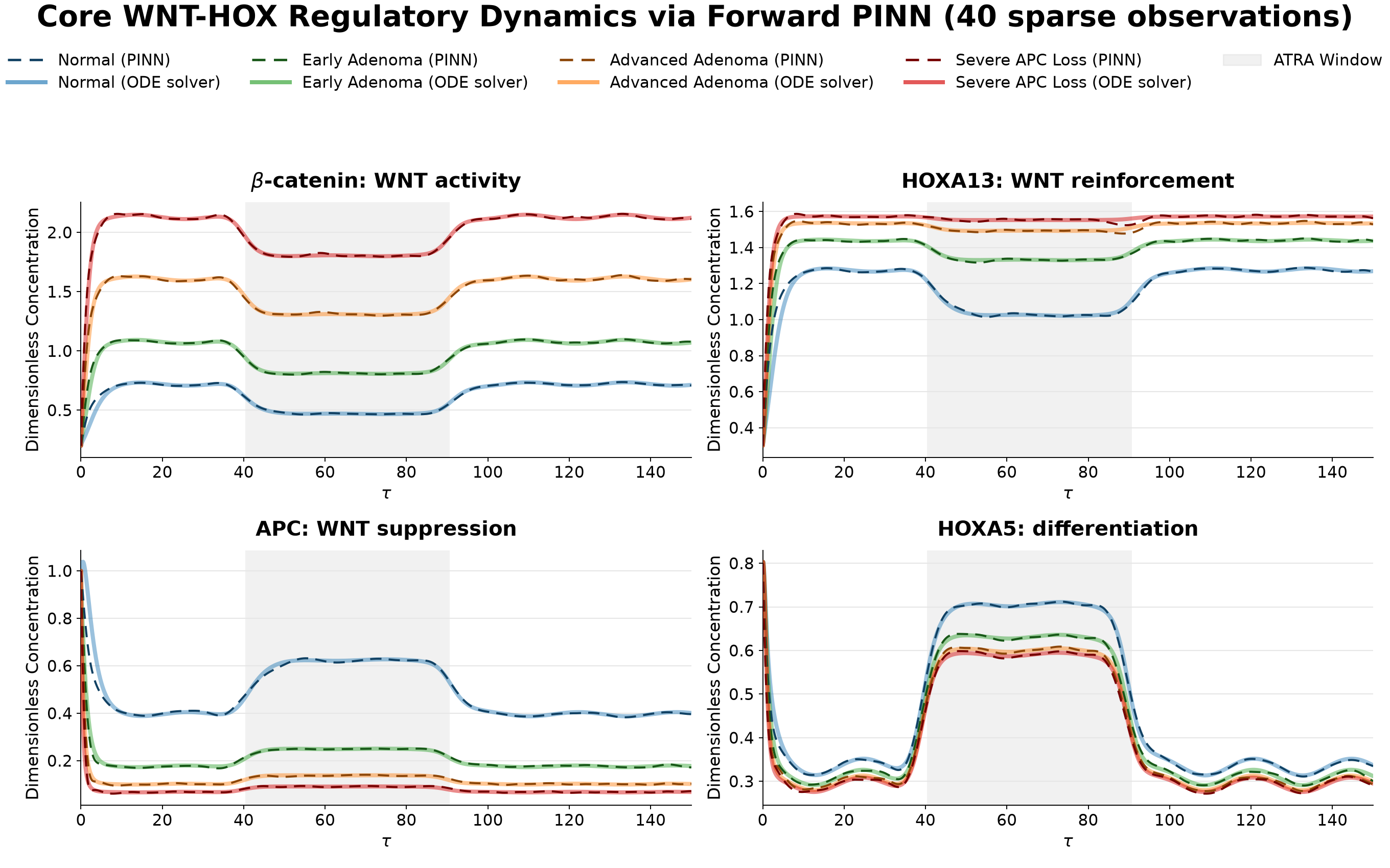
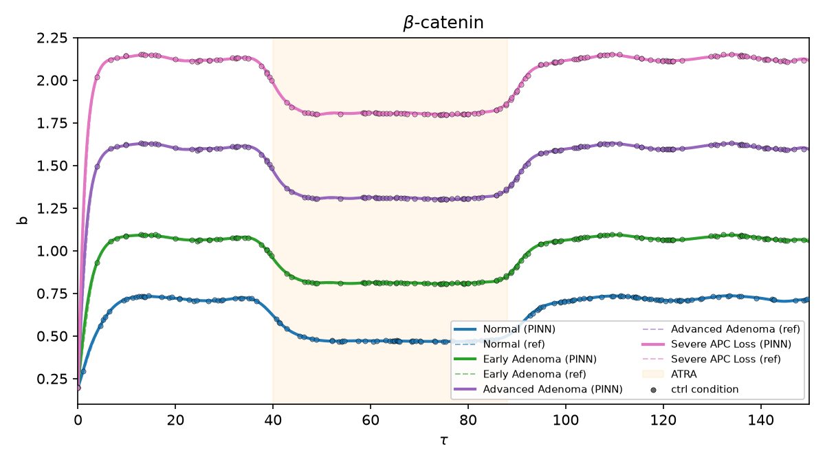
| Can a PINN reconstruct the dynamics? | The forty-observation forward model achieved 2.41% mean relative L² error across states and regimes. | No matched physics-off control isolates the residual's contribution. |
| Can it recover all thirty-six parameters? | A revised integral-residual pipeline increased recovery from 37 to 50 parameter–regime instances across four regimes. | Multiple training and forcing changes prevent attributing that increase to the residual alone. |
| Can uncertainty reveal the ambiguity? | Fisher analysis exposed an exact confounded direction; Bayesian diagnostics revealed severe overconfidence. | No inverse HMC regime passed the mixing-and-coverage gate. |
| Can a hybrid learn a biological relationship? | Several learned functions matched synthetic truth over observed inputs; targeted depletion improved selected basal parameters. | Functional and parametric errors can move in opposite directions. The strongest design predictions failed. |
The useful outcome was a more precise experimental question. When a neural term and a mechanistic parameter can compensate for each other, what observation would force them apart? Reaching the neural function's zero-input anchor helped in several cases, but only when that intervention still left the target mechanistic parameter active.
This is a chronological account of the surviving experiments, including the dead ends, corrected analyses, and later runs that changed the interpretation. The closing source map connects the reported results to code and saved artifacts. Counts refer to individual saved runs or selected restarts unless explicitly stated otherwise; they are not averages over independent repeated datasets.
Before the inverse problem
The first useful distinction in this project was between representing a trajectory and discovering the mechanism that produced it. Those sound close. In practice, a network can do the first beautifully while getting the second wrong.
The preserved notebooks show how I arrived at the seven-state experiments. A small APC–β-catenin example used a four-layer, width-64 tanh network, 30 scattered observations, and 2,000 collocation points. I first fitted the observations and initial condition, then added the differential-equation residual. That made the basic construction tangible: one network maps time to states; automatic differentiation supplies its time derivative; the equations judge whether those states evolve consistently.
There was also a much larger starting point: a Python translation of a 27-state MATLAB signaling model, followed by a windowed PINN implementation. It divided a 30,000-unit horizon into 1,000-unit windows, used a five-layer, width-128 tanh network in each window, and passed the final state forward as the next initial condition. Fourier inputs represented the periodic forcing. These are preserved implementations, not a completed accuracy benchmark: I do not have a verified error table establishing parity with MATLAB or successful training of every window.
The reduced seven-state model made it possible to examine failures systematically. I could compare a network against a conventional numerical solution, change the observations, and distinguish a representation problem from an inference problem. All results below use synthetic trajectories generated from a specified model. They test recovery when the ground truth is known; they are not estimates from patient measurements.
The system being learned
The state vector is β-catenin, APC, HOXA5, HOXA13, MYC, retinoic acid, and CYP26A1:
The equations combine three interacting motifs. β-catenin activates MYC and HOXA13, with HOXA13 feeding back into β-catenin production. RA activates HOXA5; HOXA5 supports APC and suppresses β-catenin. RA also induces CYP26A1, which clears RA. The model is a mechanistic hypothesis about those interactions, rather than a complete description of colorectal cancer.
Every equation is a balance of production and removal. Defining a Hill response as follows makes their structure easier to see:
The implemented nondimensional system is:
The timescale ratios ε determine how quickly species respond. The η coefficients set regulatory strengths; κ values locate their half-saturation scales. The exogenous WNT and MYC inputs are zero in the original experiments and become known perturbations in the experimental-design study.
RA receives a background input, a periodic contribution, and a smooth treatment pulse:
I use a horizon of 150 nondimensional time units and a periodic input with period 24. The common initial state is [0.20, 1.00, 0.80, 0.30, 0.30, 0.60, 0.40]. The base treatment window originally ended at 80; later experiments extend it from 40 to 88. The runtime values are ρ₅ = 1.10, ρB = 1.10, and ρ₁₃ = 1.30. Those values matter because the manuscript's dimensional realization and the executable configuration are not interchangeable.
Two parameters define the four simulation regimes:
| Regime | WNT drive W | APC functionality θP |
|---|---|---|
| Normal | 0.80 | 1.00 |
| Early Adenoma | 1.00 | 0.75 |
| Advanced Adenoma | 1.50 | 0.50 |
| Severe APC Loss | 2.00 | 0.25 |
These are model regimes, not clinically validated stages. The reference trajectories come from SciPy's implicit Radau solver with relative tolerance 10⁻¹⁰ and absolute tolerance 10⁻¹². A conventional solver is already effective for this small ODE system; I am not claiming that neural training is a faster way to simulate it. A separate stemness readout summarizes the modeled balance of pro-stemness and differentiation signals:
Getting the first forward PINN to work
A forward PINN receives the parameters and learns the state trajectory. My first mature implementation used a four-layer, width-256 GELU network. Its 207,879 trainable weights produce seven outputs from a 33-dimensional time embedding: normalized time together with 16 sine and 16 cosine features.
The sampled frequencies stay fixed. The motivation was concrete: a plain network was learning a smooth trend while missing the circadian ripple and treatment response. The archived plain-MLP run produced RA values spanning approximately 0.161–0.440 where the reference spanned 0.156–0.787. The Fourier model tracked the full range. However, the surviving plain run also used a horizon of 3,000 rather than 150, so this is not a clean, single-variable Fourier-feature ablation.
One early debugging episode was simpler than an optimization failure. The June 20 Fourier checkpoint had converged, but the displayed PNGs still came from the older plain network. Evaluating the checkpoint directly gave a Normal-regime data MSE of 1.45 × 10⁻⁵. The apparently failed fit was a stale visualization. That experience changed what I treated as evidence: the checkpoint, configuration, and evaluation have to describe the same run.
The more consequential issue was the training task itself. That successful checkpoint had received 3,000 labels from an already-solved trajectory. It demonstrated supervised interpolation, with a physics penalty, but it did not demonstrate learning the solution from sparse measurements. I kept it as a baseline and made the harder question explicit.
The sparse version receives 40 irregular observation times, including the initial time, and uses three losses:
The differential equation constrains the trajectory between observations. I trained with 50,000 collocation points during Adam, followed by L-BFGS, using float64. The reported forward runs use noise-free observations, 1,000 Adam epochs, and 500 outer L-BFGS steps. The later supervised baseline uses 100 evenly spaced labels; it is distinct from the original 3,000-label checkpoint.
| Regime | 100-label baseline, mean relative L² error | 40-point sparse PINN, mean relative L² error |
|---|---|---|
| Normal | 0.49% | 2.83% |
| Early Adenoma | 0.65% | 1.76% |
| Advanced Adenoma | 1.17% | 2.09% |
| Severe APC Loss | 1.91% | 2.95% |
| Across all states and regimes | 1.06% | 2.41% |

Relative error needs context. APC becomes small in the severe regime, so its relative L² error is 13.53%, while its RMSE divided by the reference range is only 1.26%. Across all species and regimes, the sparse model's range-normalized RMSE is 1.68%. I report both measures because a small denominator can make a visually accurate trajectory look disproportionately bad.
This established that the representation was useful. It did not establish the physics term's isolated contribution: a matched 40-point, physics-off control is absent. The result supports sparse reconstruction by the combined method, rather than a universal claim that the residual alone explains the improvement.
Turning the parameters into unknowns
For inverse learning, the network still maps time to states. The biological parameters become additional trainable scalars. This is not a network that receives a trajectory and directly predicts a parameter vector; each dataset gets its own optimization.
I started with only W and θP unknown, leaving all other constants fixed. There were 80 observation times with additive Gaussian noise of standard deviation 0.01 in nondimensional state units. That is an absolute noise level, not a uniform 1% relative error across species. Every regime started from W = 1.20 and θP = 0.60. Positivity and the interval constraint on θP were enforced through smooth parameter transformations.
| Regime | W relative error | θP relative error |
|---|---|---|
| Normal | 1.15% | 0.63% |
| Early Adenoma | 0.39% | 1.12% |
| Advanced Adenoma | 2.87% | 23.53% |
| Severe APC Loss | 5.12% | 141.97% |
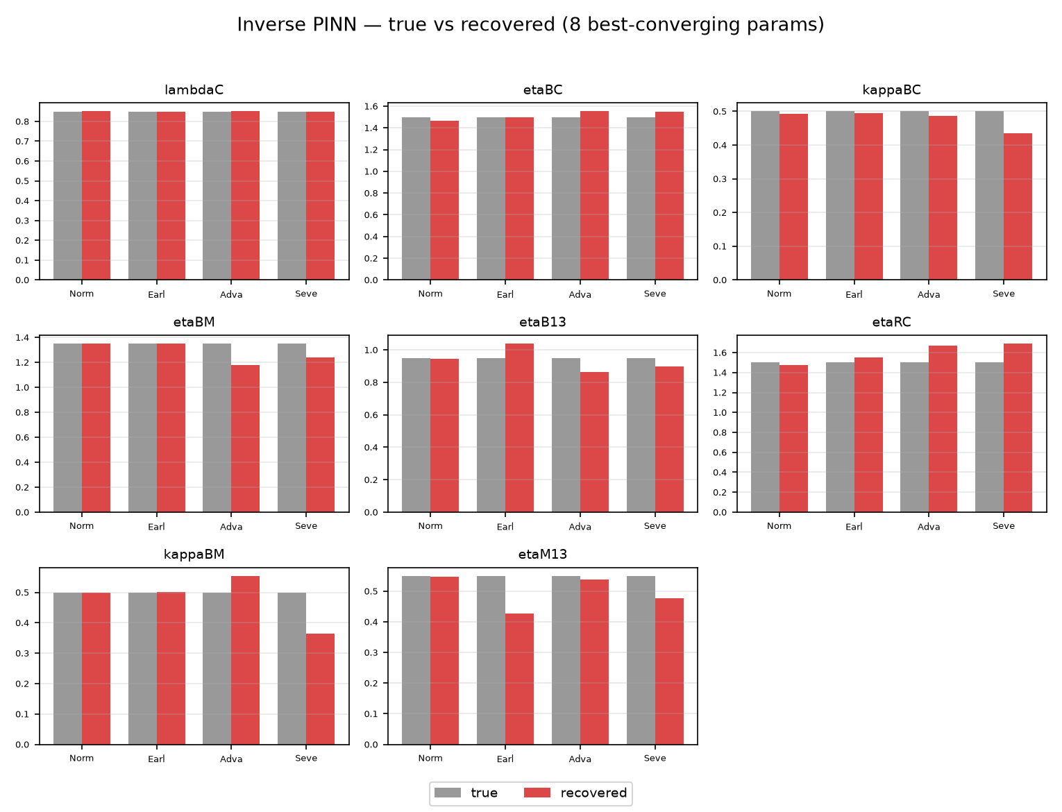
W recovered well across the four cases. In Severe APC Loss, θP barely escaped its initial guess. The difficulty therefore appeared before I asked the optimizer to estimate dozens of parameters.
There are two separate issues here. At high WNT drive, saturation and weak APC responses make the data less informative about θP: a practical identifiability problem. When δP1 is also unknown, the equations contain an exact ambiguity because APC decay depends only on δP1(1 − θP). That algebraic confounding does not explain the two-parameter experiment, where δP1 was fixed. Keeping those explanations separate is essential.
The next experiment freed all 36 continuous parameters that actually enter the residual. Hill exponents and known forcing schedules remained fixed; two auxiliary coefficients absent from the residual were excluded. Positive parameters were initially offset by 50% from baseline, with the same deliberately displaced W and θP guesses. The first single-condition run recovered only 4, 8, 7, and 7 of 36 parameters within 10%, in regime order. Average relative parameter error was approximately 47%.
The 10% threshold is a consistent score for this synthetic benchmark. It is neither a biological standard nor a proof of identifiability. A correct estimate can occur by chance; a poor estimate can reflect optimization failure, weak information, or both.
The interventions that did not solve recovery
I first improved conditioning. Positive parameters became nominal values multiplied by exponentials of trainable scalars, so updates operate on relative scales. I separated the learning-rate schedules: the earlier shared cosine schedule had driven the physical parameters toward negligible steps while the state networks were still adapting. I scaled network outputs and adjusted the physics weight using gradient norms.
I also introduced multiple experiments. Each condition gets its own state network, but all conditions share one biological parameter vector. Three RA protocols became six: control, no treatment, early treatment, late treatment, low dose, and stronger periodic forcing. A parameter estimate must now explain several trajectories under known inputs.
Those changes did not produce a steady improvement. The three-condition run recovered 8/12/6/4 parameters; six conditions recovered 10/4/5/7. More conditions were helpful only if they supplied information that the original experiment lacked.
The obvious architectural hypothesis was that the networks were too flexible. I reduced each network from 207,879 to 38,279 weights, applied weight decay of 10⁻⁴ only to network weights, and alternated five network updates with five parameter updates. Recovery became 9/10/2/4, slightly below the original six-condition total. Capacity control and alternating updates did not resolve this benchmark's inference failure.
The logs explain why I stopped treating a falling loss as sufficient progress. During a frozen-network refinement, W remained near 0.613 rather than its true 0.80 while the physics loss stayed near 4.5 × 10⁻⁵. In another experiment, networks fitted to data reached trajectory RMSE around 0.005; after freezing them, parameter fitting reduced the differential residual to approximately 2.39 × 10⁻⁴ while moving W to 0.504. The residual improved substantially and the parameter remained wrong.
Automatic differentiation was not computing an incorrect derivative. It was accurately differentiating an imperfect approximation. A small error in a function does not guarantee a small error in its derivative. When parameters are fitted against that derivative, they can compensate for its discrepancy. Joint training adds a second difficulty: the state network can reduce the residual at an incorrect parameter vector, leaving little gradient to correct the parameters. The experiments support these failure mechanisms without establishing a universal ceiling for every PINN formulation.
A classical baseline and more informative experiments
I needed an estimator that did not depend on a learned state derivative. The classical baseline integrates the ODE for each candidate parameter vector and minimizes its disagreement with observations using trust-region least squares. The implementation uses LSODA inside the fit, with log/sigmoid parameter coordinates. It recovered 18/17/13/13 parameters from the six-condition design, compared with the PINN's 10/4/5/7.
That comparison was informative precisely because the baseline was ordinary. It showed that some of the available information was being lost in the neural estimation procedure. It also showed that removing the network did not make every parameter recoverable.
The six original conditions all changed RA input. I added four protocols that directly perturb previously underexplored parts of the system:
| Added condition | Known intervention | Intended information |
|---|---|---|
| WNT pulse | +1.0 drive over time 30–70 | Move β-catenin through Hill-response transition regions |
| WNT inhibition | −0.7 drive from time 50 onward | Move high-WNT regimes away from saturation |
| MYC pulse | +1.2 drive over time 30–70 | Probe MYC regulation of the HOX species |
| WNT + RA | Sustained +0.8 WNT drive with stronger RA treatment | Probe the coupled response to both inputs |
The ten-condition classical pipeline recovered 24/23/21/14 parameters. Fourteen parameters met the 10% threshold in all four regimes. Nevertheless, Severe APC Loss remained difficult: θP error was 264%. The pipeline also added residual scaling, four restarts, and a larger least-squares budget, so the full improvement cannot be assigned to experimental design alone. The derivative-based PINN's ten-condition run reached 16/9/6/6—better overall, but still well below the classical estimator.
Replacing the differential residual
The next PINN used the integrated equation between adjacent points. Approximating the integral by the trapezoidal rule gives:
This residual uses network values without differentiating them with respect to time. Gradients with respect to trainable weights and parameters still come from backpropagation. The trapezoidal approximation has discretization error; it is not the same numerical method as the Radau reference solver.
I combined it with a fixed, sorted collocation grid, per-state relative weighting, and two starts. In this synthetic benchmark, those relative weights use the full reference trajectory, with a 0.05 scale floor; a real-data implementation would need a scale estimate available from observations. The inverse state networks use 150 observation times per condition, distinct from the forty-observation forward experiment. The selected runs recovered 17/16/10/7 parameters. The full progression makes the scale of that gain clear:
| Method | Conditions | Normal | Early | Advanced | Severe |
|---|---|---|---|---|---|
| Original inverse PINN | 1 | 4 | 8 | 7 | 7 |
| Conditioned inverse PINN | 3 | 8 | 12 | 6 | 4 |
| RA-condition PINN | 6 | 10 | 4 | 5 | 7 |
| Smaller networks + alternating updates | 6 | 9 | 10 | 2 | 4 |
| WNT/MYC-condition PINN | 10 | 16 | 9 | 6 | 6 |
| Integral-residual bundle | 10 | 17 | 16 | 10 | 7 |
| Classical ODE fit | 6 | 18 | 17 | 13 | 13 |
| Expanded classical pipeline | 10 | 24 | 23 | 21 | 14 |
Each entry counts estimates within 10% of truth, out of 36. These are archived outcomes using the seed-42 data recipe, not means over independent seed sweeps.
The closer ten-condition comparison is a total of 37 to 50 successful parameter estimates across four regimes. Calling this “the integral residual doubles recovery” would conflate the increase from six to ten conditions with the later training changes. Even 37→50 measures a bundle: the planned controls isolating relative weighting and the residual crashed, and the SIREN variant never yielded an evaluated result. The base treatment pulse also changed from ending at 80 to ending at 88. There is no completed, isolated causal estimate of the residual's contribution.

Finally, choosing the lowest physics loss was itself unreliable. In three of four regimes, that rule selected the start with fewer correctly recovered parameters. Selecting by ground-truth accuracy would have produced a total of 55, but an actual inverse problem does not reveal the truth. I therefore report the 50 selected by the prespecified loss rule. The next question was how to diagnose that ambiguity without access to the answer.
Sensitivity analysis, and a result I had to correct
Before interpreting any recovered parameter, I wanted to know which parameters moved the model's outputs. I used three complementary quantities: local normalized elasticities, Morris screening, and Sobol variance decomposition. The reduced-model screen varied 14 selected parameters and measured the time-averaged area under each state trajectory and the stemness readout over the 150-unit horizon. This is a different parameter set and question from the 36-unknown inverse problem.
Local elasticity asks how a small fractional parameter change affects a fractional output change. Morris samples elementary effects across a box, reporting their mean absolute magnitude and variability. Sobol analysis decomposes output variance under a specified input distribution: the first-order index measures the contribution of one parameter alone, and the total-order index includes its interactions. A large sensitivity index does not establish identifiability. Several sensitive parameters can still move the output in indistinguishable directions.
The first global analysis appeared to give a simple story: APC functionality dominated stemness. That story was contaminated by the sampling domain. Applying the same ±30% box to every parameter put thetaP, a functionality fraction with baseline 1, in the interval [0.70, 1.30]. With deltaP1 = 3.5, the model's APC decay becomes negative above approximately 1.286:
Those samples were testing a different dynamical regime from the intended biology. At thetaP = 1.30, the APC time-averaged AUC was roughly 6,357, compared with 0.473 at baseline. Because APC appears in the denominator of the stemness readout, the contamination propagated there too. The stored APC Sobol estimate had a first-order sum of 1.145 and a thetaP estimate of 1.146 with uncertainty ±1.198. Finite-sample Sobol estimates can leave their theoretical bounds; here the enormous uncertainty and pathological trajectories were reasons to investigate, not results to interpret biologically.
I reran the analysis with the upper limit clipped to 1.0. The script used 40 Morris trajectories (600 solves) and a Sobol base size of 256 (4,096 solves), seed 42, and LSODA with relative tolerance 1e-7 and absolute tolerance 1e-9. The correction changed the conclusion:
| Stemness statistic | Original, inadmissible box | Corrected box |
|---|---|---|
| Largest Morris mean absolute effect | θP: 1.212 | η13: 0.533 |
| Next largest corrected Morris effects | — | θP: 0.448; ηR: 0.442 |
| First-order Sobol index of θP | 0.750 | 0.154 |
| Leading corrected first-order indices | — | η13: 0.232; ηR: 0.167 |
| Parameters crossing the heuristic nonlinearity flag | 13 of 14 | 0 of 14 |
The corrected stemness first-order sum was 0.950 and the total-order sum 1.029, consistent with predominantly additive variation over this particular box. That does not make the nonlinear ODE globally linear. APC functionality remained locally influential: its stemness elasticity was about −3.61. Globally it belonged to a leading group rather than dominating alone.
There is a second qualification: clipping halved θP's sampled range while leaving the others unchanged. The before/after Sobol magnitudes refer to different input distributions. I use the correction to withdraw the original dominance claim, not to estimate an intrinsic, distribution-independent importance ranking. The saved configuration and numerical tables make that distinction reproducible.
What the data can identify
The inverse experiments left two different explanations on the table. An optimizer can fail to find parameters that the data could determine. Or the data can be unable to distinguish several parameter vectors, even with a perfect optimizer. I examined the second possibility using an exact algebraic observation, local information geometry, and profile likelihood.
An exact ambiguity in the equations
In the mechanistic model used for the 36-parameter fits, deltaP1 and thetaP enter through the single combination deltaP1 · (1 − thetaP). Within each regime, all experimental conditions share those unknowns. Any admissible pair preserving the product gives the same APC decay multiplier and therefore the same model trajectories when the other parameters are held fixed:
This is structural confounding, visible directly in the equations. In the Normal regime, the excess-decay coefficient disappears entirely at the true θP of 1. When that coefficient is fixed, as in the two-parameter proof of concept, this particular ambiguity is removed; practical loss of sensitivity and optimization difficulties can still remain. It would be incorrect to use the two-unknown product argument to explain every failure of the earlier two-parameter fit.
Beyond this analytic degeneracy, I did not complete a symbolic structural-identifiability analysis. The following diagnostics concern local or practical identifiability under specified observations, parameter coordinates, noise scales, and numerical thresholds.
Fisher information: inspect the directions, not just the diagonal
I formed central-difference sensitivities at each regime's true parameters. The rows contain all seven states at 200 times under ten conditions: 14,000 scalar observation entries for 36 unknowns. Each column is scaled into log-parameter coordinates. With assumed additive observation noise of standard deviation 0.002, the information matrix is:
This is a diagnostic observation grid, not the sparse training dataset. The implementation uses LSODA and relative central perturbations of 1e-3. Its first version read uncertainty from the diagonal of a pseudoinverse. That can be disastrously misleading: truncating a near-null eigendirection removes the very uncertainty the calculation is supposed to expose.
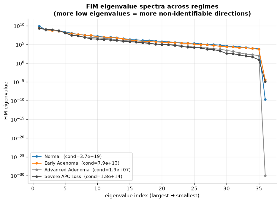
I changed the diagnostic to inspect eigenvalues and each parameter's participation in the near-null and soft subspaces. The saved run uses an eigenvalue threshold of 1 for a hard-null direction and a relative 1e-4 threshold for softer directions; these are operational numerical classifications, not universal identifiability definitions.
| Regime | Reported condition number | Hard-null directions | Pairs with absolute correlation above 0.99 | Reduced eight-parameter condition number |
|---|---|---|---|---|
| Normal | 3.7 × 10¹⁹ | 1 | 0 | 99.7 |
| Early Adenoma | 7.9 × 10¹³ | 1 | 1 | 120.9 |
| Advanced Adenoma | 1.9 × 10⁷ | 1 | 6 | 229.4 |
| Severe APC Loss | 1.8 × 10¹⁴ | 1 | 10 | 665.2 |

The exact product ambiguity appears without explicitly imposing it. Additional near-correlations involve basal production versus inducible production, and Hill amplitudes versus their thresholds. The pair count rises from 0 to 1 to 6 to 10 across the regimes. The condition number does not rise monotonically and should not be used as a disease-severity ranking. Correlations here come from an eigenvalue-floored inverse, so they are regularized local diagnostics rather than a sampled posterior.
I then fixed 28 parameters at their true values and recomputed the matrix for eight selected coordinates: lambdaC, etaBM, kappaBM, kappaBC, etaBC, etaRC, kappaB13, and kappaR. All four reduced problems had zero hard-null directions under the same criterion. This establishes that the chosen conditional subproblem is much better behaved. It does not show that those eight parameters can be learned just as well when the other 28 remain uncertain.
Profile likelihood: a useful diagnostic with an unfinished validation story
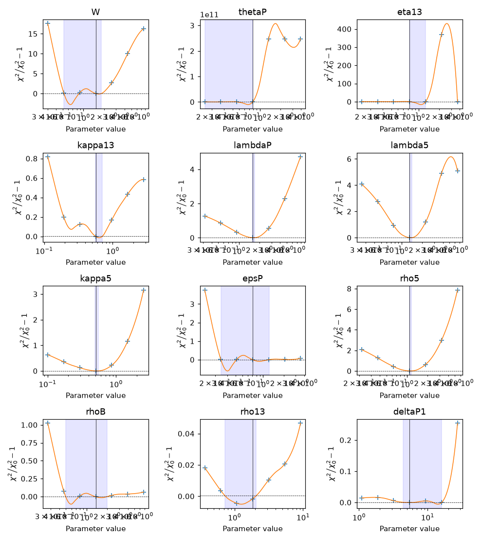
A profile scan fixes one parameter, reoptimizes the others, and records how much the fit degrades. Unlike a local quadratic approximation, it can expose asymmetric and extended valleys. I started the profiles from the excited-condition classical ODE fit and used a 25-fold logarithmic scan window.
Only Advanced Adenoma completed. Its saved classifier reports 20 parameters as identifiable and 16 as weak, with none classified as strictly non-identifiable. For example, the reported εM interval was [0.596, 0.614] around the true 0.60, whereas θP spanned roughly [0.157, 0.785] around 0.50. The original site's “16 identifiable, six marginal, fourteen not” summary does not match this completed artifact.

The numerical classification needs particular care because the algebra already proves a flat product direction. A bounded scan or imperfect nuisance optimization can manufacture finite profile intervals; several saved interval endpoints sit very close to, or even just exclude, the recorded optimum. A finite interval here cannot override an exact invariance. I treat these profiles as evidence about the implemented numerical fits, with further convergence and boundary checks needed before using them as validated confidence intervals. The Fisher code and profile artifacts preserve the actual procedures.
Bayesian inference, and the danger of confident posteriors
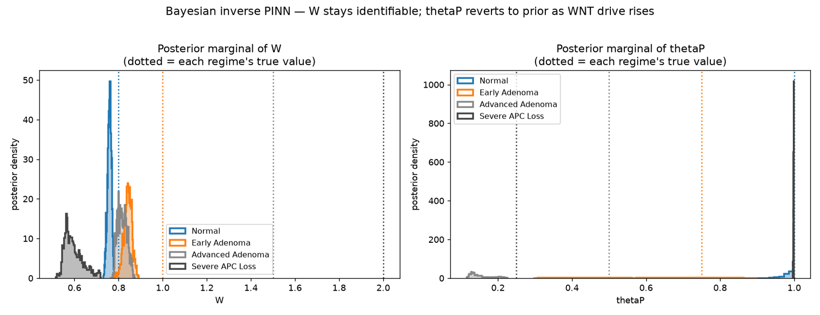
Bayesian PINNs were a natural next step: instead of one parameter vector, infer a distribution and ask whether uncertainty exposes the same ambiguities. The methodological starting point was Yang, Meng, and Karniadakis's B-PINN formulation. My implementation split the problem into two experiments. The inverse version sampled 36 physical parameters with the trained state networks frozen. The forward version held physical parameters fixed and sampled neural-network weights.
These are distinct conditional problems. In particular, the inverse version does not marginalize uncertainty in the fitted state trajectories. It should not be described as a fully joint Bayesian treatment of states and mechanisms.
The inverse sampler
I implemented Hamiltonian Monte Carlo in PyTorch with a dense mass matrix initialized from an eigenvalue-floored Hessian at the deterministic PINN estimate, warmup covariance adaptation, and dual-averaged step size targeting acceptance 0.8. Positive parameters were represented in log coordinates and θP in logit coordinates; the corresponding Gaussian prior scales were 1 and 2. Chains started from the integral-residual fit. There was one chain per regime, so no between-chain R-hat diagnostic.
Once the state networks are frozen, their direct data-fit loss is constant in the physical parameters. The parameter-dependent likelihood comes from the integral physics residual. My first implementation treated every collocation residual as an independent observation. With ten conditions, seven states, and 3,000 collocation points, that gave 209,930 residual entries, even though neighboring points lie on the same smooth fitted trajectories.
That choice allowed numerical grid density to masquerade as experimental information. Refining the grid could make the posterior sharper without collecting any additional measurements. The resulting narrow marginals looked impressive if judged only by shrinkage relative to the prior. They were not useful uncertainty estimates.
| Regime | First-run median ESS, out of 1,500 draws | Truths inside nominal 95% intervals | Naive width-based verdict |
|---|---|---|---|
| Normal | 3.4 | 1/36 | All 36 “identifiable” |
| Early Adenoma | 5.6 | 0/36 | All 36 “identifiable” |
| Advanced Adenoma | 3.1 | 1/36 | All 36 “identifiable” |
| Severe APC Loss | 5.4 | 1/36 | All 36 “identifiable” |
The median error was 29–51 posterior standard deviations from truth. Tiny posterior width was reporting a combination of a misscaled likelihood, a conditional surrogate, and a nearly stationary chain. It was not evidence that the experiment had identified every parameter.
Rescaling the likelihood improved the diagnosis, not enough to pass it
I replaced the raw residual count with a fixed effective budget: forty time samples per state and condition, giving ten × seven × forty = 2,800. The frozen inverse state networks had actually been trained with 150 observation times per condition. The forty-sample budget was a calibration choice, not a count reconstructed from that training dataset. The corrected objective weights the mean residual by the chosen budget:
For the later grid, 279,930 residual entries were downweighted by approximately 100-fold. The residual scale was calibrated at the deterministic inverse-PINN estimate used to initialize the chain, not at a separately optimized mode of the Bayesian posterior. This is a pragmatic pseudo-likelihood calibration, not a derivation proving that 2,800 residual-equivalent measurements are independent or that the resulting posterior has correct coverage.
The longer run used 3,000 warmup steps, 3,000 draws, and 48 leapfrog steps. I required median ESS of at least 200 and coverage of at least 33 of the 36 known parameter truths before accepting its identifiability labels. This was an internal synthetic-data diagnostic, not a general statistical guarantee.
| Regime | Corrected median ESS | Truths inside nominal 95% intervals | Acceptance | Gate |
|---|---|---|---|---|
| Normal | 96 | 21/36 | 0.79 | Fail |
| Early Adenoma | 1,265 | 20/36 | 0.68 | Fail |
| Advanced Adenoma | 12 | 8/36 | 0.70 | Fail |
| Severe APC Loss | 15 | 9/36 | 0.67 | Fail |

The corrected posterior means recovered 19/20/11/8 parameters within 10%, but every regime still failed the gate. Severe APC Loss was especially stark: W had posterior mean 0.596 against true 2.0, and θP was near 0.998 against true 0.25. Even the corrected sampler could be confidently wrong. Coverage was much worse in the two advanced regimes, but the sequence 21, 20, 8, 9 is not strictly monotone.
This result changed what I was willing to call a Bayesian success. A prior-shaped marginal can indicate weak information when inference is reliable. A narrow marginal from a poorly mixed or misspecified conditional calculation cannot certify identifiability. I report the saved diagnostics, not the attractive width-based labels printed beside them.
Forward uncertainty: ask what the band is supposed to cover
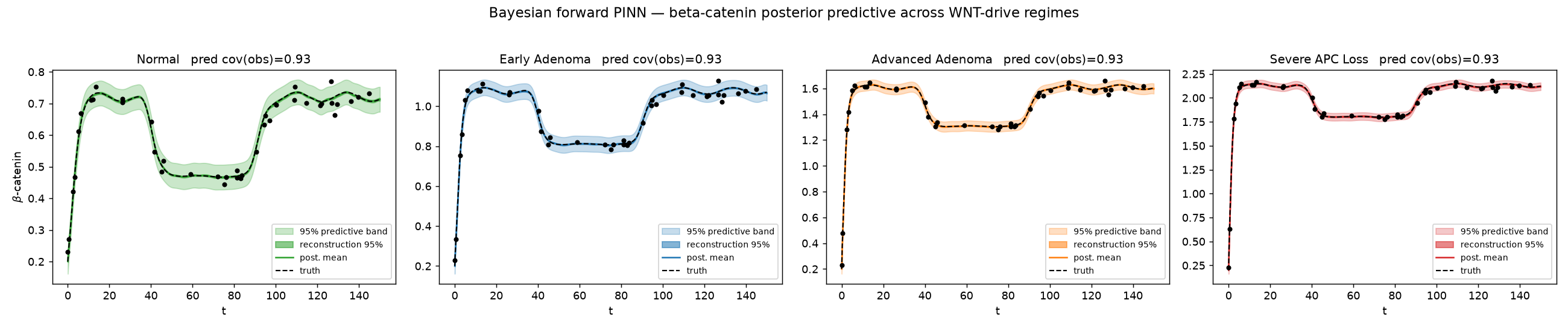
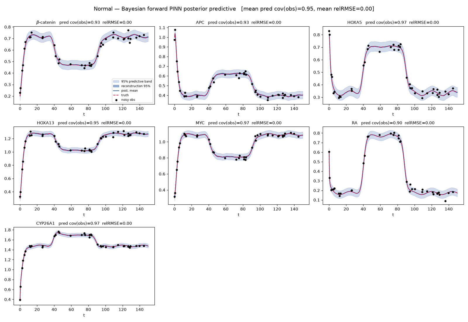
The forward experiment sampled 10,951 network weights, using a diagonal mass matrix, forty noisy observations with additive standard deviation 0.02, 800 collocation points, and 1,000 warmup plus 1,000 retained draws. The data, initial-condition, and physics likelihood scales were calibrated at an Adam-trained MAP; the recovered data scale was 0.01952 against the injected 0.02.
The first reported bands included only variation in the reconstructed function. Comparing those epistemic bands with noisy observations produced apparent coverage of 0.73/0.63/0.63/0.56. That compares different quantities. To predict a noisy observation, I needed to add observation noise to the function uncertainty:
| Regime | Predictive coverage of noisy observations | Epistemic coverage of reference trajectory | Predictive-functional ESS |
|---|---|---|---|
| Normal | 0.95 | 0.96 | 400 |
| Early Adenoma | 0.94 | 0.91 | 104 |
| Advanced Adenoma | 0.94 | 0.96 | 195 |
| Severe APC Loss | 0.95 | 0.96 | 97 |

That last qualification matters. The old article called these held-out results, but the code scores the same observations used for fitting. Also, potential-energy ESS was only 3–4 despite better ESS for the reported predictive functional. The results support an in-sample predictive check, not a claim of fully converged weight-space inference or independently validated 95% generalization coverage.
The uncertainty experiments did not solve the inverse problem. They made the distinction between a fitted curve, a fitted parameter, and a trustworthy uncertainty statement much harder to ignore.
Learning a mechanism without losing the rest of the model
The most useful result in this project came from a failed attempt to make the neural network more interpretable. I could constrain a learned regulatory function to be positive, monotone, and exactly zero at zero input—and still recover the wrong biological parameters. The constraint existed in the model. The experiments did not necessarily make it informative.
That observation changed the question. Instead of asking only which network should replace a mechanism, I began asking which experiment would let the remaining mechanism be identified after the replacement. The answer was conditional: an experiment can expose the learned function's anchor and reduce its competition with a basal-production parameter, provided the experiment still contains that parameter's contribution. Some carefully chosen interventions worked. Others reached the anchor and failed. Better recovery of a parameter did not always mean a better learned function.
Replacing one relationship at a time
The hybrid starts with the successful integral-residual inverse PINN. Each experimental condition has a state network; biological parameters are shared across conditions within a regime. I replace one selected term in the ODE with a small neural network shared across those conditions. The surrounding production, degradation, timescale, and experimental forcing terms remain explicit.
For the first experiment, the RA activation of HOXA5 changes from a Michaelis–Menten expression to a learned function:
This removes etaR and kappaR from the inverse problem. The hybrid therefore has 34 surviving mechanistic unknowns, rather than 36. Comparisons with a mechanistic control use the same 34-parameter intersection. A parameter that a network replaced cannot also count as successfully recovered. This construction belongs to the universal differential equation family; the question here is how its decomposition behaves in this particular inverse problem.
The default learned function uses two hidden layers of five tanh units, 46 trainable weights and biases in the scalar-input case. A softplus output makes the activation nonnegative, and a multiplicative gate gives it an exact zero-input anchor:
This does not tell the network the true Hill curve. It does impose a meaningful boundary condition. The neural penalty is the mean squared weight, with coefficient 1e-8 in the completed runs. Transferring regularization coefficients directly from another objective was inappropriate: coefficients of order 0.1–10 overwhelm this repository's much smaller integral-residual loss. Initialization also matters for the comparison. Constructing the learned network after the state networks preserves their random initialization across variants. The final frozen-state refinement stage made effectively no change in these completed runs; it does not explain the hybrid results.
Two recovery questions must remain separate. Parameter recovery measures relative error in the surviving mechanistic parameters, with a strict 10% cutoff for the reported counts. Functional recovery compares the learned function with the synthetic ground-truth function:
For the full PINN runs, scalar functions are evaluated on 400 equally spaced points between the minimum and maximum regulator values covered by the reference conditions. This is an error relative to the RMS of the true function, not its range. It makes no claim about extrapolation beyond that interval.
RA–HOXA5 and β-catenin–MYC: compensation is local, but the outcome is not uniform
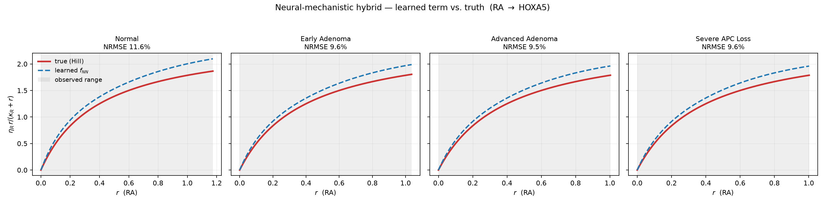
The first three-start, ten-condition comparison produced the following results. Each recovery entry is hybrid versus its control on the same 34 surviving parameters; regime order is Normal, Early Adenoma, Advanced Adenoma, Severe APC Loss.
| Replaced relationship | Recovery versus matched control | Functional NRMSE across regimes |
|---|---|---|
| RA → HOXA5, anchored | 19/18 · 17/15 · 11/11 · 6/7 | 7.6–23.7% |
| RA → HOXA5, no anchor | 18/18 · 18/15 · 10/11 · 7/7 | 3.3–24.1% |
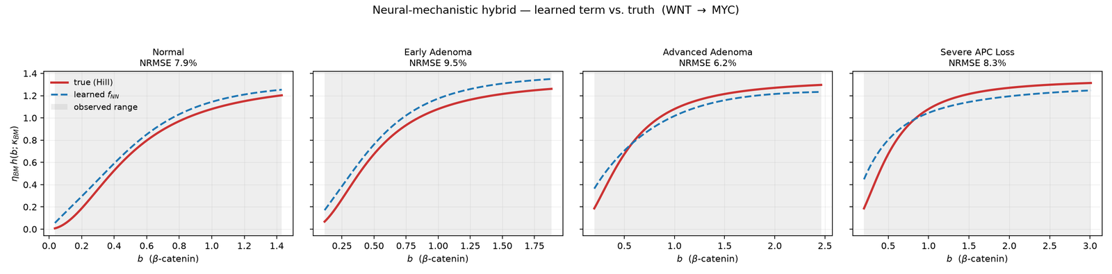
| β-catenin → MYC, anchored | 13/16 · 13/13 · 9/12 · 8/7 | 6.2–9.5% |
| β-catenin → MYC, no anchor | 13/16 · 14/13 · 9/12 · 6/7 | 8.0–13.2% |
The RA hybrid did not show the predicted overall recovery penalty: anchored and unanchored variants each recovered 53 parameters across four regimes, versus 51 for their matched control. The control itself estimated a5 poorly. Adding flexibility could improve a fit that was already difficult.
The MYC experiment more clearly exposed local compensation. It lost five recovered parameter instances overall relative to its control, four in the MYC equation. Its basal MYC parameter, aM, had 32.3% error in Normal, versus 0.4% in the control. The mechanism is visible in the equation: an additive neural term and a basal constant can trade an offset while preserving almost the same dynamics.
Both functions are zero at zero.
The measurements decide if that matters.
Away from the anchor, a changed basal rate can cancel almost the entire offset. The largest remaining production mismatch in the shaded range is 0.000.
An exact f(0)=0 rules out a global constant shift, but a flexible function can still approximate that shift over an observed interval bounded away from zero, bending back toward the anchor in the unobserved gap. For RA, the gate was already 0.70–0.76 at the lowest observed input. Neither the presence of an anchor nor a visually plausible curve established parameter identifiability.
APC: calibrate the function before inverting mutation severity
The APC experiment required a different design. Mutation severity is constant within one regime. Learning an arbitrary function of that unknown severity from one input value would confound the function and its input.
I therefore learned only excess APC degradation, retaining the healthy degradation baseline:
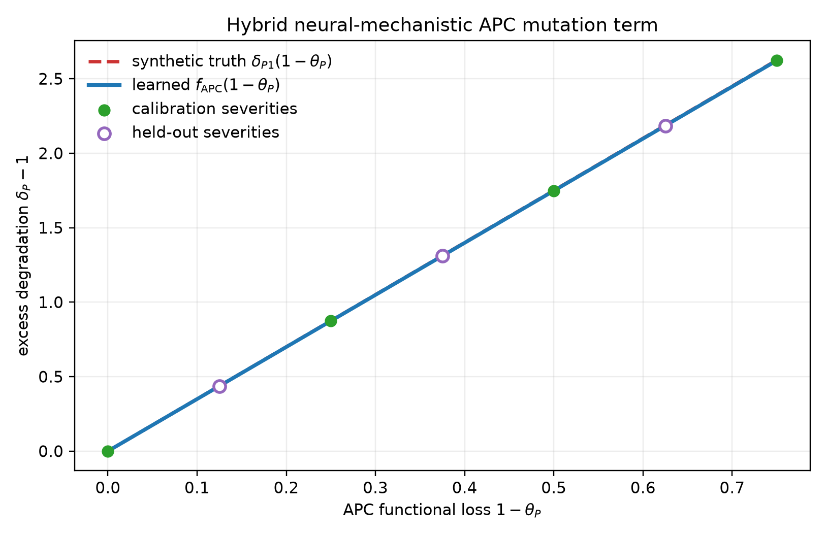
First, a shared nonnegative, monotone network was calibrated at known thetaP values 1.0, 0.75, 0.5, and 0.25. Intermediate severities 0.875, 0.625, and 0.375 were held out. Calibration used control, early-ATRA, and WNT-inhibition trajectories at fixed W=0.8, separating mutation severity from the usual regime pairing of higher WNT with greater APC loss. Then I froze the function and ran inverse PINNs with 35 mechanistic unknowns.
The held-out functional error was 0.120%; full-curve error was 0.119%. The healthy anchor was exactly zero. All five calibration starts reached closely similar physics losses. These are interpolation results for a synthetic, linear excess-degradation law under known severity labels.

The completed frozen inverse recovered 17, 15, 12, and 9 of 35 parameters, versus 18, 14, 12, and 8 for the matched control. Yet Severe APC Loss still had approximately 127% error in thetaP. A nearly exact learned function did not make its inverse input identifiable from insensitive downstream dynamics.
Screening the space of hybrid mechanisms
To investigate more mechanisms, I built a cheaper equation-local screen. It takes exact reference states, fits only the equation containing the learned term, and holds parameters outside that equation at their true values. Inside the equation, surviving parameters start near a deliberately incorrect 1.5× nominal guess. Adam followed by L-BFGS minimizes its normalized trapezoidal residual.
These screens remove state-estimation error. They are optimistic diagnostics, not full inverse-PINN results or guaranteed mathematical upper bounds. Their functional error is evaluated at sampled trajectory inputs, rather than the uniformly spaced scalar grid used above. Both changes matter when comparing absolute errors. Each screen includes its own mechanistic control.
The registry expanded to seven additive production terms, four multiplicative modulators, the three-input APC production ratio, and the separately calibrated APC mutation function. The atlas screened the twelve state-input relationships across regimes with gated and monotone constructions. The first run finished 22 Normal-regime cells and crashed on an unsupported three-input/gated pairing. A guarded restart completed the remaining three regimes; the Normal APC-production ratio cell was not completed in that atlas.
I also tested five constraint constructions on β-catenin → MYC in a separate Normal-regime screen:
| Construction | Functional NRMSE | Basal aM error |
|---|---|---|
| Positive output with exponential gate | 3.0% | 14.1% |
| Monotone function, exact anchor | 5.1% | 24.0% |
| Monotone function plus true asymptotic bound | 2.9% | 13.8% |
| Linear gate times positive learned rate | 4.8% | 22.8% |
| Linear gate times monotone learned rate | 35.1% | 202.8% |
Even the oracle upper bound did not resolve the basal error. The final construction also mismatched the target: a monotone rate multiplied by input cannot reproduce the saturating behavior in the same way as the linear APC law. More constraints can encode the wrong function class. Increasing restarts from one to two improved the gated MYC screen from 14.1% to 6.5% basal error, a larger improvement than several architecture changes.
The atlas initially suggested multiplicative modulators were easier: in Normal, all surviving host-equation parameters were recovered for the four modulators. The completed harder-regime results limited that conclusion. In Advanced and Severe regimes, the gated MYC–HOXA5 modulator had 44.7% and 46.6% functional error, while the APC–β-catenin modulator had 52.8% and 65.7%. CYP26A1-mediated RA degradation remained near 0.1%. Avoiding an additive-offset ambiguity does not remove every other source of poor recovery.
The multivariate APC production replacement was difficult too. Its monotone network had functional errors of 33.4%, 53.5%, and 16.2% in Early, Advanced, and Severe regimes, with none of the three surviving host-equation parameters below 10% error. It was scored on visited three-state combinations; filling a rectangular grid with unobserved combinations would have tested unsupported extrapolation.
Designing experiments that expose the anchor
I measured an anchor ratio, x_min / x_max, across the experimental trajectories. This is a simple diagnostic of how closely the data approach zero. It is not a universal error predictor: across the first eight RA and MYC full-PINN results, its correlation with basal error was −0.72, opposite the naive expectation. Different equations, parameter scales, and optimization outcomes confound that comparison.
The more useful test was to change the input support within matched experiments. I added a retinoid-free condition and a WNT-depletion condition. The former brought RA numerically to zero; the latter lowered β-catenin without eliminating its HOXA13 feedback-driven floor.
In one-start local screens across Normal and Severe regimes, RA → HOXA5 recovered all eight surviving host-equation parameter instances under depletion, compared with three of eight initially. RA → CYP26A1 improved from six of eight to eight of eight. The counterexample was β-catenin → CYP26A1: its basal error worsened from 24.6% to 25.5% in Normal and from 30.0% to 64.8% in Severe. Its regulator still missed zero, and a small absolute offset is a large relative error for the small basal parameter aC.
Two extra experiments also mean more information, so I added a twelve-condition comparison arm with intermediate ATRA and another WNT pulse. It matched the depletion arm's condition count without lowering regulator minima. Across four edges and two regimes, functional changes relative to the ten-condition baseline stayed between −0.4 and +0.7 percentage points; recovery counts had seven ties, one regression, and no gains. This supports the role of the chosen depletion directions. It does not make the two arms equal under every possible information measure.
An earlier attempt to use other edges as negative controls was inconclusive. One depletion directly perturbed the basal parameter of the proposed control edge; another edge was already almost perfectly recovered; the remaining MYC → HOXA13 results changed in opposite directions between regimes. That comparison could not isolate the explanation, which motivated the condition-count control.
A dose sweep tested the explanation more sharply
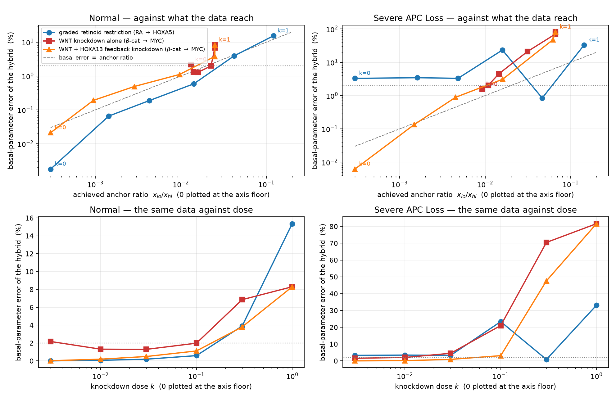
The next experiment fixed the condition count at eleven: ten baseline conditions plus one graded intervention. Three arms each used six doses, two regimes, and two restarts. RA restriction targeted the RA anchor. WNT-only depletion lowered β-catenin but left its feedback floor. A combined WNT and HOXA13-feedback knockdown removed both production routes for β-catenin.
The two β-catenin arms tested the same learned MYC term, basal parameter, optimizer, and restart seeds. Their difference was the additional feedback knockdown. At full depletion:
| Regime, original two-start sweep | WNT-only anchor ratio / aM error | Combined knockdown ratio / aM error |
|---|---|---|
| Normal | 0.0131 / 2.2% | approximately zero / rounds to 0.0% |
| Severe APC Loss | 0.0092 / 1.5% | approximately zero / rounds to 0.0% |

The local run notes recorded six predictions before the sweep. The saved scoring passed only two: the combined knockdown beating WNT-only at full depletion, and approximate cross-arm agreement at comparable anchor ratios. Monotonicity, an absolute RA error threshold, a predicted WNT-only floor above 2%, and collapse onto one shared curve did not all hold. These were exploratory recorded predictions with some inconsistent primary-versus-excess wording in the notes, not a formal external preregistration.
A completed five-start rerun of the Severe half resolved part of the optimization concern. The anomalous RA cell at dose 0.1 improved from 23.4% to 3.4% basal error. The full-dose MYC contrast persisted: WNT-only gave 2.6%, combined knockdown rounded to 0.0%. Four of six saved criteria passed in that rerun. But RA still had 3.3% basal error at full depletion, approximately matching its 3.4% mechanistic control, and its monotonicity criterion still failed. More starts improved the evidence without establishing a universal anchor-ratio law. The five-start Severe-regime plot preserves that follow-up separately from the original sweep.
A prospective failure sharpened the design rule
I then used reference trajectories, without fitting a network, to select depletion protocols for two difficult edges. Each received a baseline, a substantial intervention that missed its anchor, and the prescribed anchor-reaching intervention.
For MYC → HOXA13, the prescribed protocol drove MYC toward zero while leaving the target equation's basal a13 term active:
| Regime | Baseline a13 error | Near-miss protocol | Prescribed protocol | Functional error, baseline → prescribed |
|---|---|---|---|---|
| Normal | 12.8% | 51.5% | 0.1% | 57.2% → 68.4% |
| Severe APC Loss | 95.6% | 59.8% | rounds to 0.0% | 11.6% → 81.4% |
The basal parameter improved dramatically; the learned function deteriorated. The regulator support also changed, so these functional errors cover different sampled input distributions. The result demonstrates why a parameter-recovery success cannot stand in for functional recovery. The prediction that overall host-equation recovery would increase also failed in Severe: it remained two of four.
For HOXA13 → β-catenin, the prescribed intervention reached the anchor and did essentially nothing to W: Normal error stayed at 16.2%; Severe moved only from 57.5% to 54.7%. The reason was present in the intervention itself. Reaching that anchor required setting the WNT-drive multiplier to zero, deleting W from the very condition intended to identify it.
This leads to the narrower design rule supported by the experiments: bring the learned function's anchor into the observed support while retaining sensitivity to the mechanistic parameter it is meant to protect. The reachability checker was subsequently updated to reject protocols that switch off that basal contribution. The prospective test passed the targeted MYC basal-recovery prediction and failed broader claims about function quality and the second edge.
The resulting computational design table distinguishes several cases:
| Learned production relationship | Candidate intervention within the tested protocol ladder |
|---|---|
| RA → HOXA5 or CYP26A1 | Remove retinoid input |
| β-catenin → MYC, HOXA13, or CYP26A1 | Suppress WNT drive and HOXA13 feedback |
| MYC → HOXA13 | Also suppress basal MYC production |
| HOXA13 → β-catenin | No usable protocol in this ladder: reaching the anchor also removes W |
These are reachability prescriptions, not confirmation that every listed hybrid was trained under its prescribed intervention. APC's own state remained above zero under the tested ladder because its production term retains a positive baseline. A diagnostic computed from known reference dynamics is useful here; applying it to biology with uncertain dynamics would require additional validation.
Returning to the full inverse PINN
The later three-start, twelve-condition full-PINN runs also completed. Their absolute results are more modest than the exact-state screens:
| Learned term with depletion | Recovery / matched control, each out of 34 | Functional NRMSE | Basal error by regime |
|---|---|---|---|
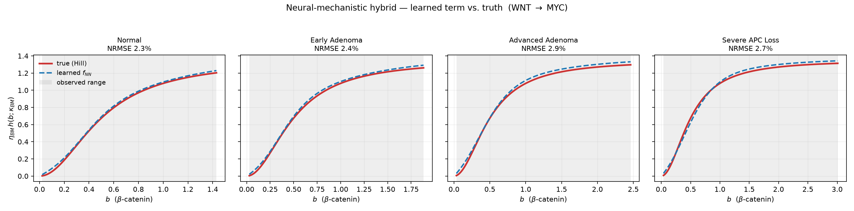
| β-catenin → MYC | 15/17 · 16/16 · 13/13 · 13/13 | 2.3–2.9% | 10.3%, 11.7%, 17.4%, 16.4% |
| RA → HOXA5 | 18/18 · 20/17 · 18/14 · 18/14 | 9.5–11.6% | 13.0%, 4.7%, 2.4%, 3.8% |
The RA hybrid gained eleven recovered parameter instances across four regimes against its same-condition, same-parameter control. Its Normal basal estimate was worse than the control, while the other three were better. The MYC function improved substantially over the original ten-condition run, but its basal errors remained much larger than its control's roughly 0.2–0.5%. Its regulator still did not reach zero in this twelve-condition protocol. The high-WNT thetaP problem persisted for both hybrids. The RA–HOXA5 learned curves show the corresponding full-PINN result alongside the MYC figure below.

All of these results come from one synthetic seven-state model with known generating equations. The local screens remove measurement and state-estimation difficulties; the full runs restore only the particular sparse-data and optimization setting tested here. Idealized knockdown multipliers are proposed computational interventions, not demonstrated laboratory protocols. The contribution is a reproducible investigation of where the hybrid decomposition fails, a useful experiment-design diagnostic, and clear counterexamples to its strongest interpretations—not a general solution to identifiability.
What I would trust, and what I would test next
The project supports a useful forward approximation and several reproducible diagnoses of inverse failure. It does not establish recovery of all thirty-six parameters, clinical validity of the model, or a general superiority of PINNs over classical ODE fitting. In this small system, classical integration is inexpensive and remains an essential baseline. Classical methods can also support Bayesian inference and neural differential equations; those extensions are not exclusive advantages of PINNs.
The most concrete mechanistic conclusion is the exact deltaP1 · (1 − thetaP) ambiguity. Reparameterizing that pair into its identifiable combination, or fixing one member using independent information, would address a structural problem that extra optimizer steps cannot resolve. It would still leave practical uncertainty in high-WNT dynamics and compensation elsewhere in the model.
The most useful experimental-design lesson is narrower than “observe near zero.” An intervention must change the support of the learned function while preserving the contribution of the parameter it is intended to identify. A condition that removes both the neural input and the basal parameter cannot separate them. The failed HOXA13-to-β-catenin protocol made that distinction explicit.
The next experiments I would prioritize follow directly from the limitations. First, isolate the integral residual with identical data, pulse schedules, weighting, initialization, and computational budgets. Second, repeat the strongest comparisons across independent noise draws and seeds, reporting distributions rather than the best run. Third, evaluate the hybrid designs under noisy or partial state observations and uncertainty about the generating model. Fourth, rerun the Bayesian work with multiple chains, explicit trajectory uncertainty, and genuinely held-out predictive checks. These are proposed tests, not completed results.
There is also a practical lesson in the experiment infrastructure. Separate timestamped run directories preserved failed variants and checkpoints. Long jobs ran in tmux; queues moved through conditions and regimes without relying on an open SSH connection. But persistence alone did not make a run trustworthy: stale plots, incomplete atlas cells, a failed ablation, and malformed aggregate logs all required returning to the saved numerical outputs. The reportable unit is the configuration, fitted artifact, evaluation rule, and result together.
I started by asking whether a neural network could solve the equations. The more revealing question became whether the observations could determine the explanation I was asking the network to learn. A good fit was the beginning of that investigation.
Sources and reproducibility
The PINN-Research repository contains the model, experiment implementations, analyses, and manuscript. This account was checked against the repository and saved run artifacts on September 10, 2026. The pre-hybrid manuscript and historical notes occasionally retain claims superseded by later artifacts; the numerical scopes and qualifications above take precedence in this article.
The article's evidence record lists exact source paths, run identifiers, important corrections, and figure provenance. The repository tracks the cited numerical runs; dated working notes remain local. The evidence record distinguishes those sources. The figures shown here are copied from those saved outputs; the cover and interactive anchor example are explicitly illustrative.
| Part of the investigation | Implementation and evidence |
|---|---|
| Early models and first PINNs | Original notebooks in notebooks/ and PINN/; forward implementations |
| Two-parameter and full inverse learning | Historical PINN-inverse-solve/, then multi-condition training and its architecture variants |
| Classical estimation and excitation | WNT/MYC experimental conditions and ODE fitting |
| Integral-residual training | PINN-inverse-pinn-boost |
| Sensitivity and identifiability | Sensitivity script, full Fisher analysis, and reduced Fisher analysis |
| Bayesian calibration | Inverse HMC and forward HMC |
| Hybrid mechanisms and experimental design | Hybrid implementation, edge screens, and reachability checks |
The work builds on established methods. Raissi, Perdikaris, and Karniadakis developed the PINN framework used as the starting point. Yang, Meng, and Karniadakis formulate Bayesian PINNs. Rackauckas and colleagues describe universal differential equations combining known dynamics with trainable components. These references establish the methodological context; they do not validate this model's biological assumptions or imply priority for the experimental-design observations reported here.
This article documents my implementation and experiments within the collaborative project. The reduced model and associated write-up are work with Nate Kim and our advisor. Questions about the analysis or reproducing a particular run are welcome at aaidark1@swarthmore.edu.